You can download here the figures of the book. Simply click on the figure to retrieve a pdf file with the caption.
You can also retrieve all the figure as a single zip file.
Figures from chapters 1 to 11 can be reproduced using the Wavelab Matlab toolbox. The Wavelab directory has a folder called WaveTour. It contains a subdirectory for each chapter WTCh01, WTCh02, ...) ; these subdirectories include all the files needed to reproduce the computational figures from chapters 1 to 11. Each directory has a demo file.
Many of the figures of the books (including most of the numerical experiments of chapters 12 and 13) can be obtained by going through the numerical tours.
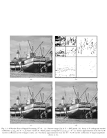 Fig.1.1: Linear vs. non-linear approximation |
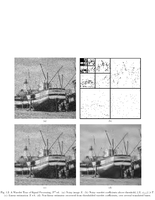 Fig.1.2: Denoising by wavelet thresholding |
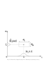 Fig.1.3: Heisenberg box representing a Gabor atom |
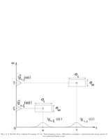 Fig.1.4: Time-frequency boxes representing the energy spread of two windowed Fourier atoms. |
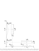 Fig.1.5: Heisenberg time-frequency boxes of two wavelets |
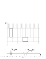 Fig.1.6: The time-frequency boxes of a wavelet basis define a tiling of the time-frequency plane |
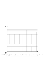 Fig.1.7: A wavelet packet basis divides the frequency axis in separate intervals of varying sizes. |
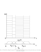 Fig.1.8: A local cosine basis divides the time axis with smooth windows |
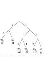 Fig.10.1: Prefix tree |
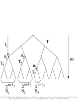 Fig.10.2: Coding tree |
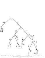 Fig.10.3: Huffman tree |
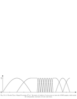 Fig.10.4: Adapted windows |
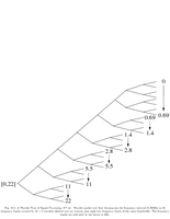 Fig.10.5: Wavelet packet tree |
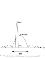 Fig.10.6: Audio coding |
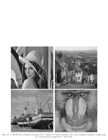 Fig.10.7: Wavelet compression with adaptive arithmetic coding |
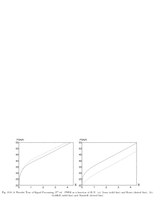 Fig.10.8: Rate distortion for image coding |
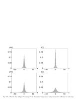 Fig.10.9: Histogram for wavelet coefficients |
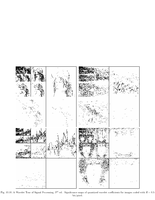 Fig.10.10: Significance map |
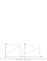 Fig.10.11: Rate distortion for wavelet coding |
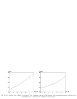 Fig.10.12: SPIHT embedded code |
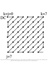 Fig.10.13: Block of cosine coefficients |
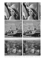 Fig.10.14: JPEG compression |
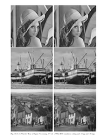 Fig.10.15: JPEG-2000 compression |
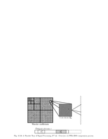 Fig.10.16: JPEG-2000 process |
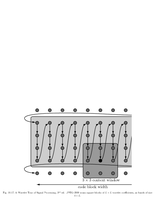 Fig.10.17: JPEG-2000 ordering |
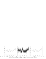 Fig.11.1: Gaussian process denoising |
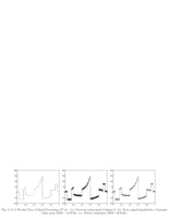 Fig.11.2: Piecewise smooth signal Wiener denoising |
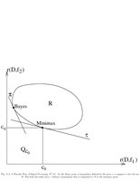 Fig.11.3: Bayes vs. minimax |
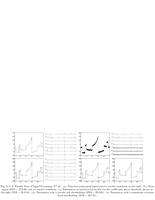 Fig.11.4: Piewise smooth wavelet denoising. |
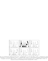 Fig.11.5: Sure denoising |
 Fig.11.6: Curvelet denoising |
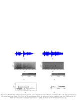 Fig.11.7: Audio denoising |
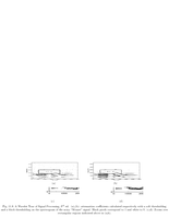 Fig.11.8: Audio block denoising |
 Fig.11.9: Audio block denoising |
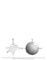 Fig.11.10: Orthosymmetric set |
 Fig.12.1: Wavelet packet tree |
 Fig.12.2: Best wavelet packet basis |
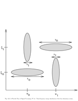 Fig.12.3: Time frequency distribution of a signal |
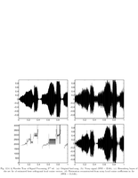 Fig.12.4: Best cosine basis |
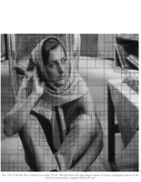 Fig.12.5: Best cosine basis for an image |
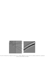 Fig.12.6: Wavelet coefficients as samples of a regularized function |
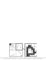 Fig.12.7: Bandlet quadtree |
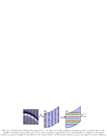 Fig.12.8: Wavelet coefficient for bandletization |
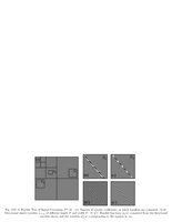 Fig.12.9: Discrete bandlets |
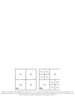 Fig.12.10: Construction of a dyadic segmentation |
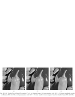 Fig.12.11: Bandlet approximation |
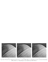 Fig.12.12: Bandlet denoising |
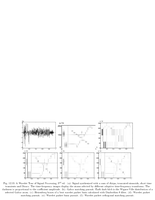 Fig.12.13: Matching and basis pursuit in wavelet packet dictionary |
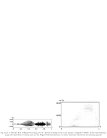 Fig.12.14: Matching pursuit for audio signal |
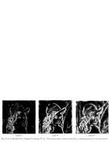 Fig.12.15: Directional Gabor wavelet pursuit |
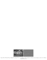 Fig.12.16: Video coding |
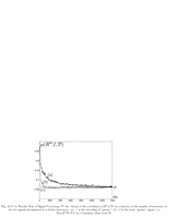 Fig.12.17: Correlation decay during matching pursuit |
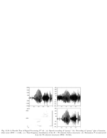 Fig.12.18: Coherent structures by pursuit |
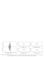 Fig.12.19: Marching vs. basis pursuit in Gabor |
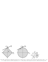 Fig.12.20: Geometry of L1 minimization |
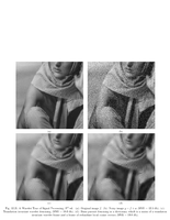 Fig.12.21: Denoising of an image in a redundant dictionary |
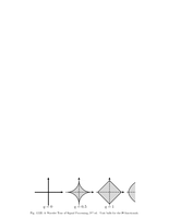 Fig.12.22: Unit balls |
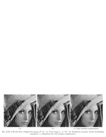 Fig.12.23: Total variation regularization |
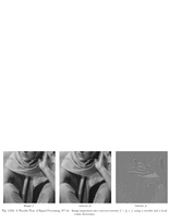 Fig.12.24: Image separation |
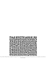 Fig.12.25: Dictionary learning |
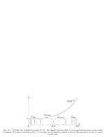 Fig.13.1: Mirror wavelets |
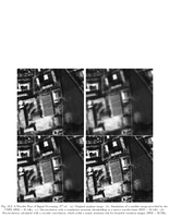 Fig.13.2: Satellite image deblurring |
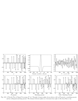 Fig.13.3: Sparse spikes deconvolution |
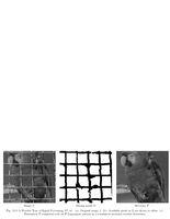 Fig.13.4: Inpainting using wavelet regularization |
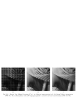 Fig.13.5: Sparse superresolution |
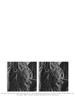 Fig.13.6: Super resolution by directional interpolation |
 Fig.13.7: Tomography inversion |
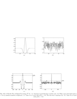 Fig.13.8: Sparse spikes filters |
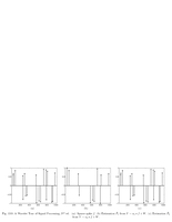 Fig.13.9: Seismic filters |
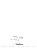 Fig.13.10: Compressed sensing recovery of sparse signals |
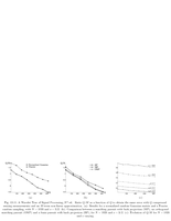 Fig.13.11: Compressed sensing recovery of compressible signals |
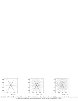 Fig.13.12: Blind source separation geometry |
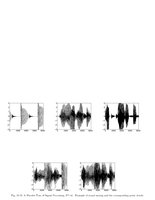 Fig.13.13: Blind source separation |
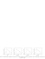 Fig.2.1: Gibbs oscillations |
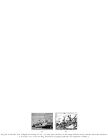 Fig.2.2: Total variation. |
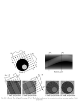 Fig.2.3: Radon transform |
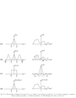 Fig.3.1: Shannon Theorem |
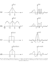 Fig.3.2: Aliasing |
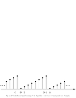 Fig.3.3: Periodization |
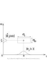 Fig.4.1: Heisenberg box of a Gabor atoms |
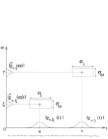 Fig.4.2: Heisenberg boxes of two Gabor atoms |
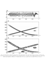 Fig.4.3: Linear and quadratic shirps and modulated Gaussian |
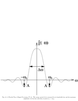 Fig.4.4: Window design |
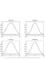 Fig.4.5: Four windows |
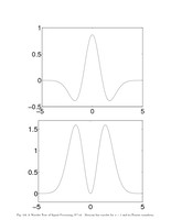 Fig.4.6: Mexican hat |
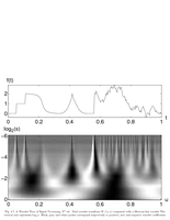 Fig.4.7: Mexican hat wavelet transform |
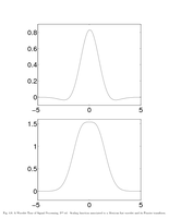 Fig.4.8: Scaling function of mexican hat wavelet |
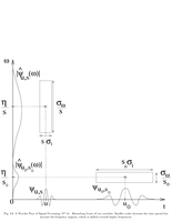 Fig.4.9: Heisenberg boxes of two wavelets |
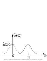 Fig.4.10: Fourier transform of a wavelet |
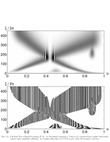 Fig.4.11: Scalogram |
 Fig.4.12: Ridges of a chirp |
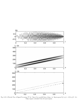 Fig.4.13: Ridges of chirps |
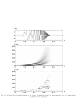 Fig.4.14: Sum of two hyperbolic chirps |
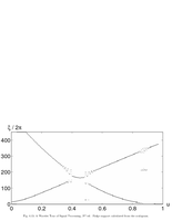 Fig.4.15: Ridge support computed from scalogram |
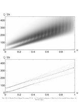 Fig.4.16: Scalogram of two parallel linear chirps |
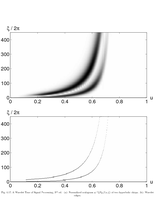 Fig.4.17: Scalogram of two hyperbolic chirps |
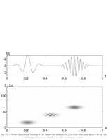 Fig.4.18: Wigner-Ville distribution of two Gabors |
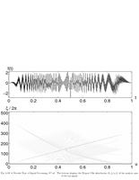 Fig.4.19: Wigner-Ville distribution of a signal |
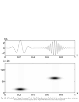 Fig.4.20: Choi-William distribution of two Gabor |
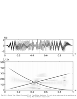 Fig.4.21: Choi-William distribution of a signal |
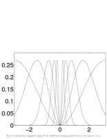 Fig.5.1: Fourier transform of wavelets |
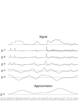 Fig.5.2: Dyadic wavelet transform |
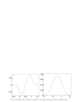 Fig.5.3: Quadratic spline wavelet and scaling function |
 Fig.5.4: Dyadic wavelet filters and reconstruction |
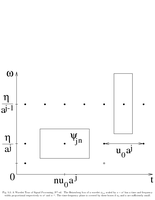 Fig.5.5: Heisenberg box of a wavelet |
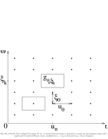 Fig.5.6: Windowed Fourier frame |
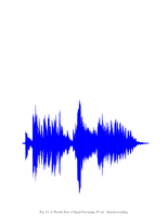 Fig.5.7: Musical recording |
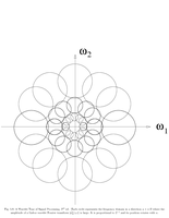 Fig.5.8: Oriented wavelets |
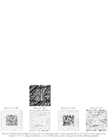 Fig.5.9: Directional Gabor |
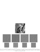 Fig.5.10: Steerable pyramid |
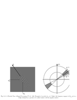 Fig.5.11: Curvelets and its Fourier transform |
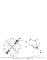 Fig.5.12: Spacial and Fourier tiling of curvelets |
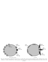 Fig.5.13: Layout of wavelets and curvelets around an edge |
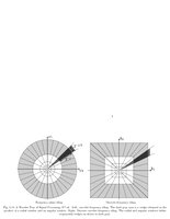 Fig.5.14: Curvelet frequency tiling. |
 Fig.6.1: Wavelet transform with derivated of Gaussigna. |
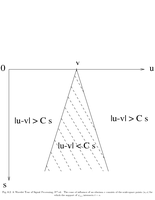 Fig.6.2: Cone of singularities |
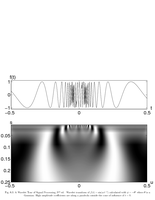 Fig.6.3: Cone of oscillating singularity |
 Fig.6.4: Wavelet transform of a discontinuitiy |
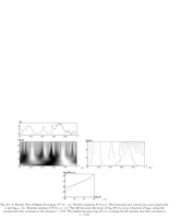 Fig.6.5: Modulus maxima |
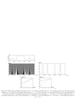 Fig.6.6: Decay of wavelet coefficient along maxima curves |
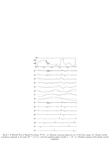 Fig.6.7: Dyadic modulus maxima |
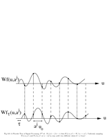 Fig.6.8: Translation invariance of wavelets |
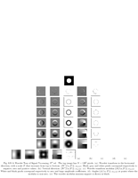 Fig.6.9: |
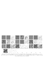 Fig.6.10: Oriented wavelet transform and modulus maxima |
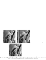 Fig.6.11: Reconstruction from wavelet maxima |
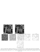 Fig.6.12: Restauration from thresholded maxima |
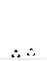 Fig.6.13: Kaniza illusory contours |
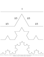 Fig.6.14: Von Koch subdivision |
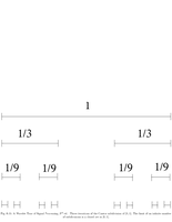 Fig.6.15: Cantor set |
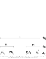 Fig.6.16: Cantor measure |
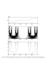 Fig.6.17: Devil staircase |
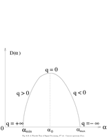 Fig.6.18: Concave spectrum |
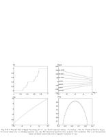 Fig.6.19: Devil staircase spectrum |
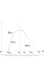 Fig.6.20: Spectrum of a perturbation |
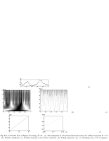 Fig.6.21: Brownian motion |
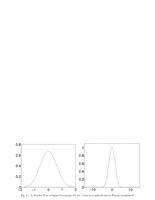 Fig.7.1: Cubic box spline |
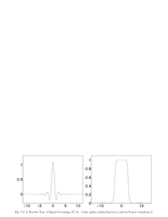 Fig.7.2: Cubic spline scaling function |
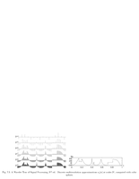 Fig.7.3: Discrete multiresolution approximation |
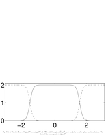 Fig.7.4: Cubic spline filters |
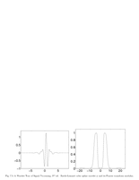 Fig.7.5: Barrle-Lemarie cubic spline |
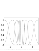 Fig.7.6: Fourier transform of the Battle-Lemarie spline wavelets |
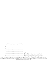 Fig.7.7: Wavelet coefficients for cubic spline wavelets |
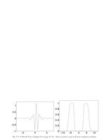 Fig.7.8: Meyer Wavelets |
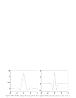 Fig.7.9: Linear spline Battle-Lemarie |
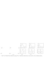 Fig.7.10: Daubechies scaling function |
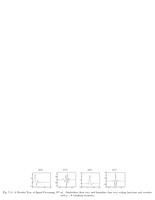 Fig.7.11: Daubechies and Symmlets scaling functions and wavelets |
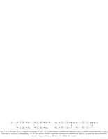 Fig.7.12: Fast wavelet transform |
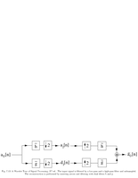 Fig.7.13: Wavelet reconstruction |
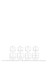 Fig.7.14: Spline biorthogonal wavelets and scaling functions |
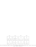 Fig.7.15: Biorthogonal wavelets and scaling functions |
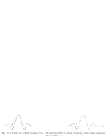 Fig.7.16: Periodic wavelet |
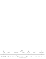 Fig.7.17: Folded signal |
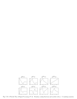 Fig.7.18: Boundary scaling function and wavelets |
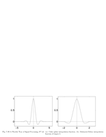 Fig.7.19: Cubic spline interpolation functions |
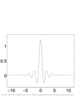 Fig.7.20: Dual cubic spline for interpolation |
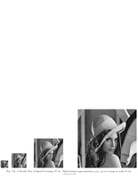 Fig.7.21: Multiresolution image approximation |
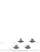 Fig.7.22: Fourier transform of a separable wavelet transform |
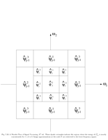 Fig.7.23: Fourier support of 2D wavelets |
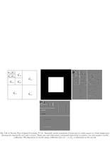 Fig.7.24: Separable wavelet transform of Lena |
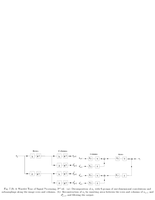 Fig.7.25: Fast 2D wavelet transform |
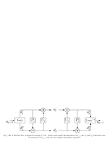 Fig.7.26: Predict and update lifting |
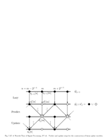 Fig.7.27: Predict and update for linear wavelet lifting |
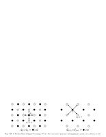 Fig.7.28: Quincunx subsampling |
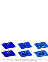 Fig.7.29: Quincunx wavelets |
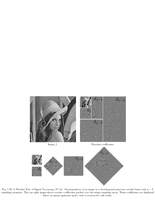 Fig.7.30: Decomposition of an image in a biorthogonal quincunx wavelet |
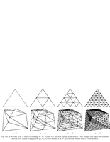 Fig.7.31: Triangular mesh subsampling |
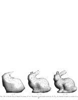 Fig.7.32: Example of semi-regular mesh |
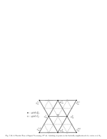 Fig.7.33: Labeling of points in butterfly scheme |
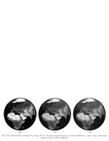 Fig.7.34: Non-linear approximation of a function on the sphere |
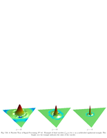 Fig.7.35: Dual wavelet on a triangles |
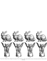 Fig.7.36: Non-linear surface approximation |
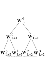 Fig.8.1: Binary wavelet packet tree |
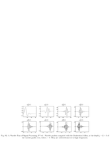 Fig.8.2: Wavelet packet with Daubechies filters |
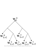 Fig.8.3: Admissible packet tree |
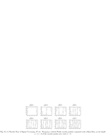 Fig.8.4: Walsh packets |
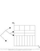 Fig.8.5: Heisenberg box of wavelet packets |
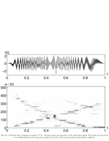 Fig.8.6: Multi-chirp signal decomposed in wavelet packets |
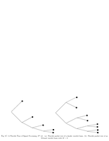 Fig.8.7: Dyadic wavelet basis tree. |
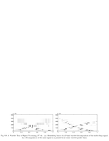 Fig.8.8: Multi-chirp decomposition in cosine wavelet packet |
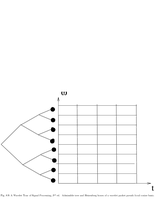 Fig.8.9: Admissible tree and Heisenberg box |
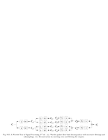 Fig.8.10: Wavelet packet analysis and synthesis |
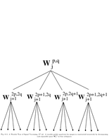 Fig.8.11: Wavelet packet quad tree |
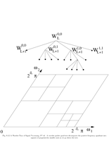 Fig.8.12: Wavelet packet frequency decomposition |
 Fig.8.13: Wavelet packet decomposition in 2D |
 Fig.8.14: Symmetric extension |
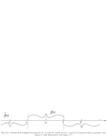 Fig.8.15: Cosine IV |
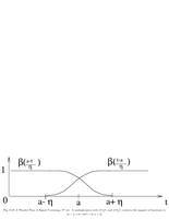 Fig.8.16: Lapper projector |
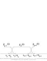 Fig.8.17: Local cosine windows |
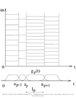 Fig.8.18: Local DCT Heisenberg boxes |
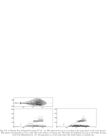 Fig.8.19: Local cosine audio decomposition |
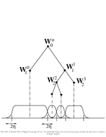 Fig.8.20: Local cosine admissible tree |
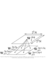 Fig.8.21: Local cosine windows |
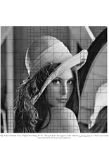 Fig.8.22: Local cosine image subdivision |
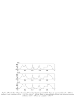 Fig.9.1: Fourier vs. Wavelets approximation |
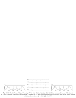 Fig.9.2: Non-linear wavelet approximation |
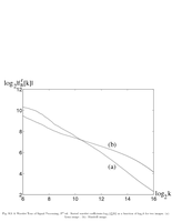 Fig.9.3: Approximation curves |
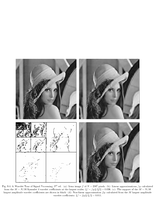 Fig.9.4: Linear vs. non-linear approximation |
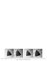 Fig.9.5: Approximation using triangulation |
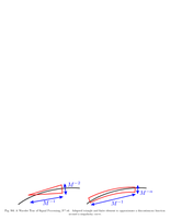 Fig.9.6: Adapted finite element approximation |
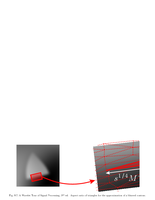 Fig.9.7: Aspect ratio of triangles |